
Loan Loss Provisions Are Not Enough to Protect the Bank
This is Article 3 of 5 in the Q-Lana Risk Management series. Loan loss provisions cover expected loss, while equity capital covers the tail. A 100-loan simulation shows losses have a floor but no ceiling, and that capital rises faster than confidence.

Loan loss provisions are not enough on their own. They cover the average year, while equity capital covers the bad one. A bank can enter a downturn with provisions booked correctly and coverage ratios within policy. Its expected loss calculation may be beyond criticism. Then defaults rise, and the provisions run out. This is rarely negligence. It comes from a misunderstanding of what provisions are designed to do, which a normal year never exposes.
What Are Loan Loss Provisions Designed to Cover?
Expected loss (EL) is what the bank anticipates losing in an average year. Unexpected loss (UL) is how far actual losses can deviate from that average. Provisions absorb the first, and equity capital absorbs the second.
Many credit committees review provision coverage every month. Far fewer discuss how much capital sits behind the book. A bank that manages only provisions is prepared for the years that were never the problem. Under IFRS 9 expected credit loss rules, provisions are forward-looking. An institution that has thought hard about one and not the other is prepared for the years that were never the problem.
Reading the Loss Distribution
Picture the full range of credit losses your portfolio could produce next year as a curve.
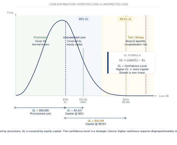
Frequent losses and tail losses
Losses up to expected loss are frequent and unremarkable. Provisions handle them. Larger losses sit in the tail of the distribution. Equity capital covers them, up to a confidence level the bank chooses or the regulator sets.
Choosing a confidence level
The confidence level turns a statistical idea into a management decision. Once it is set, the capital question becomes a distance question. How far beyond expected loss must the bank be able to absorb? Roughly two standard deviations covers about 95 per cent of outcomes. Getting to 99.9 per cent takes more than three. The capital charge for unexpected loss is, in essence, a multiple of the volatility around the expected loss, and the multiple is set by an appetite decision rather than by mathematics. The Basel IRB formulas apply the same logic. The size of the buffer is an appetite decision, and the mathematics only measures it.
What a Simulation of Loan Loss Provisions Shows

The previous article used a portfolio of 100 identical loans. Running 10,000 simulated years against that portfolio shows how losses actually spread.
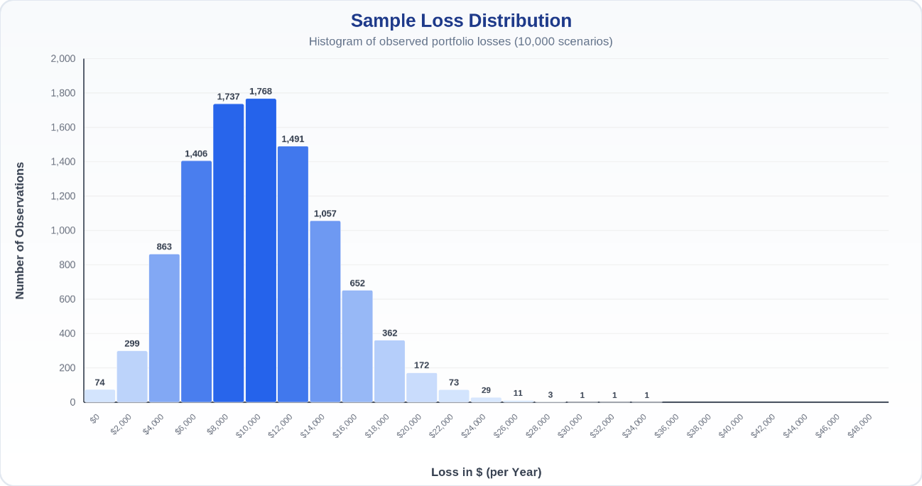
The chart above presents the outcomes of a sample Monte Carlo simulation used to analyze potential losses in a loan portfolio. If you replicate this simulation, the exact results will likely differ due to the inherent variability in random sampling. However, the key patterns and insights remain consistent across simulations.
The most common outcome is the expected loss
Total losses of 10,000, meaning five defaults, occurred in 1,768 of the 10,000 runs. The average is genuinely the single most likely result, which is what makes it so persuasive and so incomplete.
The upside is capped
In 4,379 runs, fewer than five loans defaulted. In 74 runs, none did. The best possible year saves you the whole $10,000 and no more, because losses cannot go below zero.
The downside is not
In theory, all 100 loans could default. One run produced 17 defaults, a loss far above expectation.
That asymmetry is the entire subject. A credit portfolio has a floor and no ceiling. Good years are bounded; bad years are not. Any risk framework built on averages is implicitly assuming a symmetry that does not exist.
Reading the Percentiles
The simulation gives loss levels at each confidence level, and unexpected loss is simply the distance between that level and the expected loss.
|
Confidence level |
Portfolio loss |
Unexpected loss |
Losses exceed this |
|
90% |
14,621 |
4,621 |
1 year in 10 |
|
95% |
16,305 |
6,305 |
1 year in 20 |
|
99% |
20,153 |
10,153 |
1 year in 100 |
|
99.9% |
24,019 |
14,019 |
1 year in 1,000 |
At the 90th percentile, losses reach $14,621. Unexpected loss is $4,621.
At the 95th, $16,305, so unexpected loss is $6,305.
At the 99th, $20,153, so unexpected loss is $10,153, which is now larger than the expected loss itself.
At the 99.9th, $24,019, so unexpected loss is $14,019.
Two things are worth sitting with in that sequence:
i. The confidence level is a real choice with a real price
Covering 95% of years means being wrong roughly once in twenty. Covering 99.9% means being wrong once in a thousand. A conservative institution holds more capital and accepts lower returns on it. A more aggressive one holds less and accepts a higher chance of recapitalization. Both are legitimate positions and neither is an accident.
ii. Capital grows non-linearly with confidence
Moving from 95% to 99% costs roughly another $4,000 of capital on this portfolio. Moving from 99% to 99.9% costs another $10,000. The same one-notch improvement in resilience costs two and a half times as much at the higher level, because the tail is thin and getting further into it is expensive.
What does this mean for risk appetite?
This non-linearity matters most to anyone setting risk appetite. The question is never simply whether to be prudent. It is what the next step of prudence costs. The board then has to decide whether that capital could earn more elsewhere.
Losses up to the expected loss are covered by provisions. Losses beyond it are covered by equity, and the confidence level you choose decides how much. Capital is not a compliance output. It is the price of the certainty you selected.
Building this in your team
The Q-Lana Financial Skills Campus runs a credit risk measurement course for credit teams and risk functions, covering rating and scoring design, calibration to observed default rates, and how the three variables connect through to pricing and capital. Taught on your own portfolio rather than on textbook cases.
Where the Simple Model Stops
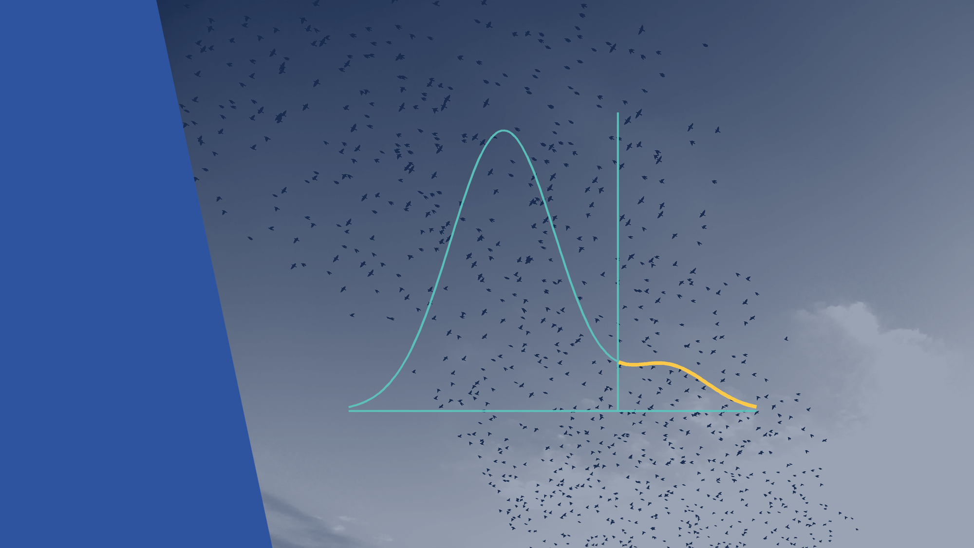
The simulation above assumes a homogeneous portfolio of identical, independent loans. Real portfolios are neither, and four factors change the answer.
i. Heterogeneity
Loans differ in size, risk, collateral and borrower. Loan-level adjustment is required, and concentration in a few large exposures fattens the tail well beyond what an average-based model suggests.
ii. Correlation
This is the important one. Defaults cluster. Borrowers fail together when a sector contracts or a macroeconomic shock lands, because they are exposed to the same conditions. Independence is a convenient assumption and a false one, and every point of correlation moves capital more than an equivalent move in the average probability does.
iii. Stress testing
Simulations describe the distribution you can infer from history. Stress tests ask what happens under scenarios history has not yet supplied, a different, complementary question.
iv. Advanced modelling
Monte Carlo is a robust foundation. Large, diverse books eventually need copula models or richer stress frameworks to represent dependency properly.
None of that argues against starting simple. It argues against stopping there, and against reporting a tail number without stating the correlation assumption that produced it.
Three Changes to How Banks Report Loan Loss Provisions and Capital
None of these changes requires rebuilding a model.
i. State the confidence level
A capital figure quoted without a confidence level means little. A bank that has never chosen its level still has one, usually inherited from a regulatory minimum. In that case, nobody actually made the decision.
ii. Report provisions and capital separately
Provisions and capital answer different questions and should not be discussed in the same breath as though they were interchangeable buffers.
iii. Treat a good year with caution
Suppose losses come in at $7,000 against an expected $10,000. The $3,000 difference looks like a surplus. Paying it out as profit reduces resilience. That decision is often made without anyone describing it in those terms.
Next in This Series
The next article, takes this from portfolio level down to the individual loan, which is where capital becomes a number a relationship manager can actually influence.
Explore the Loss Distribution
The asymmetry in this article is far more convincing when you move the inputs yourself, particularly the correlation coefficient, which visibly fattens the tail while the average stays exactly where it was. Please have a look at our interactive loss distribution explorer and test your scenarios
Q-Lana · Risk Management
Interactive Loss Distribution Explorer
One hundred loans, fifty thousand simulations. Move a parameter and watch expected loss, unexpected loss and the capital requirement respond.
Portfolio Parameters
Confidence Level
Key Metrics
Non-Linear Capital Requirement
| Confidence | VaR | UL / Capital | Capital % | Marginal Cost |
|---|
If you are interested to read more Background and the concepts including the simulation results and the capital implications, read the Q-Lana white paper Credit Risk and Risk Appetite.
All the Articles in This Series:
- Credit Risk Measurement Should Come Before Instinct
- Expected Loss Is a Cost Every Loan Must Cover
- Loan Loss Provisions Enough to Protect the Bank (this article)
- Is Loan-Level Capital a Constraint or a Signal?
- RAROC Separates Good Lending From Profitable Lending
Follow Q-Lana
One short email a week on credit risk, lending and impact finance, free. Or browse more guides in the Q-Lana Knowledge Center.
Get Q-Lana Weekly
One short email a week on credit risk, lending and impact finance, free. Or browse more guides in the Q-Lana Knowledge Center.