Credit Risk

Expected Loss in Credit Risk: Formula, Calculation & Examples

This is the second article in our Credit Risk Management series, introducing Expected Loss and its role in measuring average credit losses. We explain how EL is calculated and how it connects to Unexpected Loss and risk variability.

Kenneth Ochieng 29 April 2025 5 min read

Expected Loss in Credit Risk: Formula, Calculation & Examples

Expected Loss (EL) represents the average level of credit losses a financial institution anticipates over a given time horizon, typically one year.

It quantifies the cost of bearing credit risk and is a foundational concept in pricing loans, setting provisions, and managing portfolios.

Each component (Probability of Default (PD), Loss Given Default (LGD), and Exposure at Default (EAD)) provides a distinct perspective on risk, and their combination offers a comprehensive view of expected credit loss.

What Is Expected Loss (EL)?

Expected Loss is a cost. It is comparable to an insurance premium. Just as insurance companies calculate premiums to cover anticipated claims, financial institutions use EL to estimate the average losses they might incur from defaults in their loan portfolios.

EL = PD × LGD × EAD

Expected Loss in Loan Loss Provisions

Expected loss allows financial institutions to:

1. Calculate Provisions and Reserves

EL guides the allocation of provisions to ensure the institution is prepared for average losses, acting as a buffer against expected defaults.

2. Calculate Loan Pricing

EL influences loan pricing, as it represents the cost of credit risk. If the calculated EL for a loan is $100, this amount must be factored into the loan's interest rate or fees.

3. Risk Management

Institutions use EL to monitor portfolio health; if EL increases due to rising PDs or LGDs, it may signal deteriorating credit quality.

Limitations of Expected Loss

EL is not an indication of risk and uncertainty. It does not account for variability or extreme outcomes, which are addressed by Unexpected Loss (UL).

Calculating Expected Loss Step By Step

Consider a loan portfolio of 100 homogenous loans, each: loan amount $10,000, 4-year term with linear amortization, PD of 5%, collateral value $3,000, default occurring on average after 2 years.

Calculating EL for an Individual Loan

Step 1

Estimate EAD: with linear amortization, exposure at the midpoint (two years) is 50% of the original loan.

EAD = 0.5 × 10,000 = 5,000.

Step 2

Estimate LGD: with a collateral value of $3,000 against an exposure of $5,000, the lender loses $2,000, so LGD is 40%.

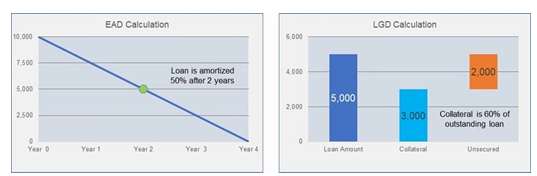
Using the input to calculate, Expected Loss for a single loan results in $100.

EL (Individual Loan) = 10,000 × 5% × 40% × 50% = $100.

What is the actual loss if one loan defaults?

This question differs from the EL calculation because it assumes that the borrower has already defaulted removing the probability component. For a loan amount of $10,000, an EAD of 50% ($5,000), and an LGD of 40%, the loss is:

Loss in Default = 10,000 × 40% × 50% = $2,000, irrespective of the probability of default.

What is the expected loss of the total portfolio?

We know that there are 100 homogeneous loans in the portfolio. The EL for an individual loan is $100. Multiply by the total number of loans in the portfolio:

EL (Portfolio) = EL (Individual Loan) × 100 = 10, 000

The total expected loss for the portfolio is $10,000

What Happens When Reality Deviates from Expectations

While Expected Loss provides an average estimate, real-world defaults often deviate from expected values due to their probabilistic nature. Let us explore two scenarios where the actual default rate differs from the expected 5%.

Scenario 1: Fewer Defaults Than Expected (4%)

If only 4% of loans default instead of 5%, the number of defaults in a portfolio of 100 loans is 4. The loss per defaulted loan is $2,000 (as calculated earlier), so the total loss is:

4 × 2, 000 = 8, 000

With provisions of $10,000 set aside, the institution has a surplus of $2,000, which could be retained as additional reserves. However, in many cases, institutions may treat this surplus as profit, distributing it as dividends or bonuses to shareholders and staff.

Scenario 2: Higher Defaults Than Expected (6%)

If the default rate increases to 6%, the number of defaults in the portfolio is 6. The total loss increases to:

In this case, the institution’s provisions of $10,000 fall short by $2,000. This shortfall must be covered by equity capital, underscoring the importance of maintaining an adequate capital buffer to absorb such unexpected losses.

What Causes Deviations in Portfolio Losses?

Real-world portfolios rarely conform strictly to expected default rates. Variability can arise from economic conditions (recessions increase defaults; growth reduces them), model accuracy (poor calibration of PD or other variables skews projections), and default range (if defaults range from 3% to 7%, portfolio losses would vary between $6,000 and $14,000): underscoring the importance of robust provisioning strategies and regular stress testing.

Complex Portfolios: How Do You Deal With Them?

In addition to these variations, there are other aspects to consider in a more complex assessment:

Heterogeneous Portfolios: For portfolios with diverse loan structures, collateral types, or borrower profiles, EL must be calculated for each loan or segment and then aggregated.
Dynamic LGD and EAD: Factors like collateral depreciation, legal delays, or unexpected drawdowns can alter LGD and EAD over time, requiring regular reassessment.
Correlation Effects: While EL assumes independent defaults, real-world portfolios often exhibit correlation (e.g., defaults clustering during economic downturns). EL itself does not account for these dynamics but is a key input for more complex risk models, including stress tests and scenario analyses.

Bridging to Unexpected Loss

Expected Loss gives you the average, but not the whole picture. The financial institution must also account for Unexpected Loss (UL), which captures variability and ensures capital adequacy during periods of higher-than-expected defaults.

Q-Lana calculates Expected Loss and Unexpected Loss automatically at both the loan and portfolio level, and feeds the results directly into RAROC and risk appetite reporting. See the platform →

In the next chapter, we explore how UL builds on EL to provide a comprehensive view of credit risk and inform decisions on capital allocation.

About This Series

This article is part of Q-Lana's Credit Risk Concepts series, exploring the quantitative techniques that support pricing, capital planning, and performance measurement.