Credit Risk

Unexpected Loss (UL): Capital Buffers, Calculation & Portfolio Implications

This is the third chapter of our credit risk series where we build on the previous discussion of expected loss, introducing unexpected loss, which is the more volatile, less predictable side of credit risk.

Kenneth Ochieng 15 April 2025 7 min read

Unexpected Loss (UL): Capital Buffers, Calculation & Portfolio Implications

While Expected Loss (EL) tells us what we anticipate losing on average, Unexpected Loss (UL) is all about uncertainty. It captures the volatility and potential deviation from that average—especially during economic stress or unexpected events. UL represents the portion of credit loss that exceeds expectations and requires capital buffers, not just provisions, to ensure institutional resilience.

Unlike EL, which is typically covered by loan loss reserves, UL must be absorbed by equity capital. It is a crucial concept for regulatory capital planning, stress testing, and maintaining the financial health of a lending institution.

What is Unexpected Loss in Credit Risk?

UL represents the potential for losses that exceed the expected loss. It accounts for:

Volatility in default rates: Unexpected increases in defaults during economic downturns.
Correlation effects: Simultaneous defaults within a portfolio due to shared risk factors.
Tail risks: Rare but severe events, such as financial crises, can cause losses far exceeding normal expectations.

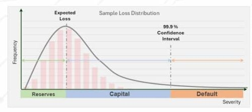
The relationship between UL and EL can be visualized as part of the loss distribution curve, where losses up to the EL are covered by provisions. Losses beyond the EL are covered by equity capital, up to a confidence level defined by the institution or regulatory requirements.

Visualizing Unexpected Loss: The Loss Distribution Curve and Confidence Levels

Imagine a bell curve representing potential credit losses.

Losses up to the Expected Loss (EL) are frequent and covered by provisions.
Losses beyond the EL—the tail of the distribution—are covered by equity capital, up to a confidence level set by the institution or mandated by regulators.

This confidence level (e.g., 95%, 99%, 99.9%) determines how much capital is required to ensure solvency in most scenarios, even extreme ones.

Modelling Unexpected Loss with Monte Carlo Simulations

To understand and quantify UL, financial institutions often rely on Monte Carlo simulations. These simulations model thousands of potential default scenarios to estimate the distribution of losses in a portfolio.

Example Portfolio Setup:

Number of loans: 100 Loan size: $10,000 each Expected Loss (EL): $10,000 (as calculated in Chapter 3) Simulation runs: 10,000 iterations

Each iteration represents a single year in the portfolio’s life, with the number of defaults and associated losses varying based on random sampling of probabilities.

Modeling Unexpected Loss with Monte Carlo Simulations

Interpreting UL Outcomes

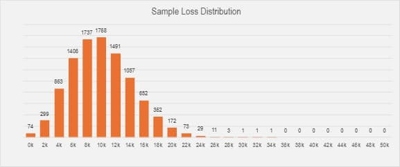
The chart above presents the outcomes of a sample Monte Carlo simulation used to analyze potential losses in a loan portfolio. If you replicate this simulation, the exact results will likely differ due to the inherent variability in random sampling. However, the key patterns and insights remain consistent across simulations.

Let us break down the main observations from this specific example:

i. Most frequent loss

In this simulation, the most common outcome, or mode, corresponds to a total loss of $10,000, which aligns with the Expected Loss (EL) derived from the default rate of 5%. This scenario assumes that 5 loans out of 100 default within the year, and it occurred in 1,768 out of 10,000 iterations.

ii. Distribution characteristics

The loss distribution observed in this simulation exhibits notable characteristics:

Limited Upside:

The distribution has a limited upside, meaning that losses are constrained below the Expected Loss when fewer than 5 loans default.

In this simulation:

4,379 cases (approximately 43.8% of all simulations) resulted in fewer than 5 defaults. Notably, 74 iterations experienced no defaults at all, demonstrating the possibility of extremely favorable outcomes, albeit infrequent.

Significant Downside:

The downside risk is more pronounced, as up to 100 loans could theoretically default in the most extreme scenarios. While rare, 1 instance was observed where 17 loans defaulted, representing a loss significantly higher than the Expected Loss. This highlights the asymmetric risk inherent in credit portfolios: while the likelihood of fewer defaults is capped, extreme losses, though rare, can be substantial

iii. Loss Percentiles and Risk Thresholds

The simulation provides insight into loss percentiles, which are critical for understanding risk thresholds and planning capital reserves:

90th Percentile: At the 90th percentile, losses reached $14,621. This indicates that in 90% of cases, the portfolio’s total losses remained below this value.
9th Percentile: At the 99.9th percentile, total losses increased to $24,019. Such losses occur in only 1 out of 1,000 years or 0.1% of the time, representing extreme scenarios.

iv. Confidence Intervals and Risk Tolerance

Financial institutions and regulators use confidence intervals to define acceptable risk levels and determine the necessary capital buffers to absorb potential losses. Common confidence levels include:

95% Confidence Level: Losses are covered in 19 out of 20 years, requiring sufficient reserves to handle losses at or below the 95th percentile.
9% Confidence Level: Losses are covered in 999 out of 1,000 years, representing a highly conservative standard often mandated by regulators for systemic stability. This level accounts for rare but severe loss scenarios.

v. Calculating Unexpected Loss from Simulation Results

The Unexpected Loss (UL) is the difference between the loss at the chosen confidence level and the Expected Loss (EL).

UL = Loss of Confidence Level – EL

For instance:

At the 90th percentile, UL = $14,621 − $10,000 = $4,621.
At the 99.9th percentile, UL = $24,019 − $10,000 = $14,019.

This calculation underscores the importance of maintaining adequate equity capital to cover these unexpected losses

Practical Implications of the UL

Understanding and managing Unexpected Loss (UL) is a cornerstone of maintaining the financial health and resilience of any institution. While reserves derived from Expected Loss (EL) cover routine, predictable losses, equity capital is specifically scaled to handle the unpredictability of UL. The level of equity capital required is directly influenced by the chosen confidence level, a measure of how much risk the institution is prepared to withstand. Losses that exceed this confidence level can lead to defaults, potentially requiring recapitalization to restore stability and ensure operational continuity.

i. Capital Adequacy

UL calculations are fundamental to defining regulatory capital requirements, enabling financial institutions to endure significant losses without jeopardizing solvency. The ability to maintain sufficient equity capital is a critical safeguard against systemic risks, ensuring long-term financial stability.

ii. Risk Appetite

Institutions operate within regulatory frameworks but have room to adjust their confidence levels based on their risk tolerance.

For example, a conservative institution may adopt a 99.9% confidence level, ensuring it is prepared for all but the most extreme loss scenarios by holding higher levels of capital. Conversely, a more aggressive institution might select a 95% confidence level, opting for lower capital reserves and accepting a greater degree of risk in exchange for potential profitability.

iii. Disproportionate Capital Increases

As confidence levels increase, capital requirements grow nonlinearly. This is evident in the Monte Carlo simulation example, where the total losses are divided into EL and UL: Increasing from 95% to 99% confidence requires an additional $4,000 in equity capital.

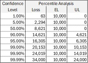
Moving further from 99% to 99.9% confidence demands another $10,000 in capital. This non-linear growth underscores the need for institutions to carefully balance their confidence levels against operational costs and risk appetite.

Simplifications and Advanced Considerations

While the calculations above are based on a homogeneous portfolio with identical loans for simplicity, real-world portfolios are far more complex. To address this, additional factors must be considered:

i. Portfolio Heterogeneity

Loans within a portfolio typically differ in size, risk profile, collateral type, and borrower characteristics. Such variations necessitate loan-specific adjustments to better reflect the portfolio’s true risk.

ii. Correlation Effects

Defaults are often not independent but may cluster due to economic downturns, sector-specific risks, or external shocks. These correlation effects can amplify losses beyond what simple models predict, necessitating more advanced risk modeling techniques.

iii. Stress Testing

Institutions frequently conduct stress tests to evaluate the impact of extreme scenarios that go beyond standard loss distributions. These tests allow institutions to assess their vulnerability to events like severe economic recessions or sudden market disruptions.

iv. Advanced Modeling

While Monte Carlo simulations provide a robust foundation, more sophisticated tools, such as copula models or enhanced stress-testing frameworks, are necessary for managing the complexities of large, diverse portfolios.

Having explored UL at the portfolio level, the logical next step is to allocate capital requirements to individual loans. This involves incorporating granular factors such as borrower specific credit risk profiles, the quality, type, and enforceability of collateral, and the effects of loan duration and maturity on risk exposure.

Q-Lana models EL and UL at the individual loan and portfolio level, with outputs feeding directly into capital allocation and risk appetite dashboards.

What's Next: How to Allocate UL to Individual Loans

In the next chapter, we will examine how regulatory frameworks like Basel III and IV provide guidance for calculating capital adequacy at the individual loan level. This enables institutions to enhance risk-adjusted pricing, optimize portfolio management, and align with regulatory expectations.

Linking UL to specific loans enables financial institutions to achieve a higher level of precision and control in their risk management practices.

About This Series

This article is part of Q-Lana's Credit Risk Concepts series, exploring the quantitative techniques that support pricing, capital planning, and performance measurement.